Haggai Maron and Yaron Lipman, Weizmann Institute of Science

This is the first post summarizing the main ideas and constructions in a series of three recent papers (Maron et al., 2019 a,b,c) introducing and investigating a novel type of neural networks for learning irregular data such as graphs and hypergraphs. In this post we focus on (Maron et al., 2019a) that was presented at ICLR 2019

Algebraic view of convolutional neural networks.

The goal of this note is presenting a family of neural network architectures suitable for learning irregular data in the form of graphs, or more generally, hypergraphs. This family presents a tradeoff between expressivity (i.e., the ability to approximate a large and complicated set of functions), and efficiency (i.e., the amount of time and space resources used by these architectures).

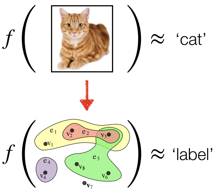
Image credit: hypergraph - Wikipedia

The main idea (see image above) is to adapt the concept of image convolutions, as a means of dramatically reducing the number of parameters in a neural network, to graph and hypergraph data. In more detail, translations of images are transformations $T$ that do not change the image content, see e.g., the image below. Hence, most functions $f$ one is interested to learn on images, like image classification, will be invariant to translations, namely will satisfy $f(x)=f(T\cdot x)$ for all translations $T$, where $x$ represents the image, and $T$ the application of the translation to the image.

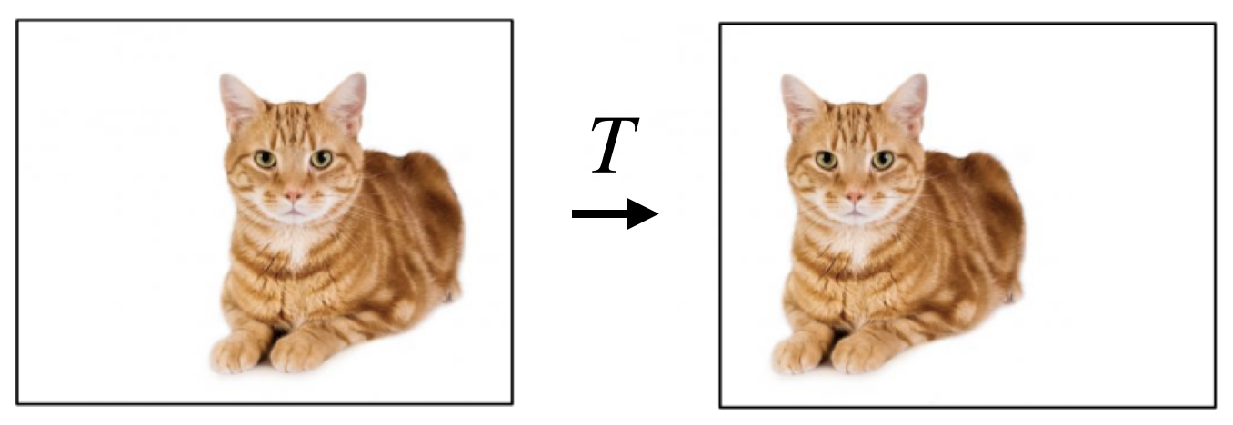
Image credit: imgur - https://imgur.com/mEIUqT8

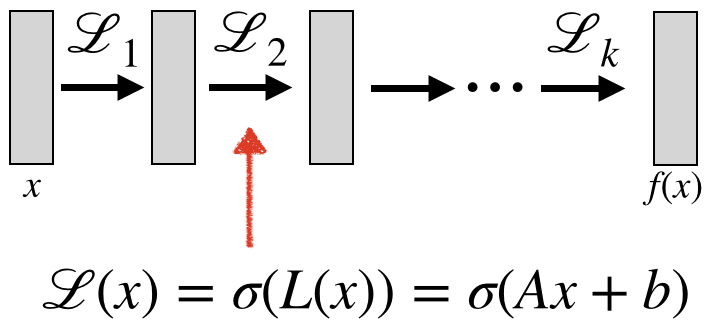
A Multi-Layer perceptron (MLP) is a general-purpose architecture that can approximate any continuous function (Cybenko 1989, Hornik 1991). The architecture is composed of multiple layers $\mathcal{L}_i$, where each layer has the form $\mathcal{L}(x)=\sigma(L(x))$, where $x$ is the input to the layers, $\sigma$ is a non-linear function applied entry-wise (e.g., ReLU), and $L(x)=Ax+b$ is a linear (in fact, affine) function. $A,b$ are the tuneable parameters of the network. Using an MLP to learn functions on images is daunting: consider a low-resolution image of $100\times 100 \times 3$, and let the output of the first layer be of the same dimension $100\times 100\times 3$ (say we want to apply some transformations to the colors of the image). This would make the parameter of dimension $10^9$ (approximately) and would only represent the linear part of a single layer.

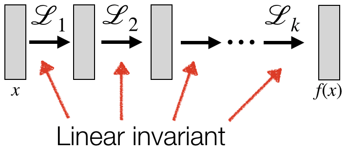
Motivated by the fact that we are looking to approximate invariant functions, a reasonable way to try and reduce this huge number of parameters, is to replace the general linear (in fact, affine) transformations $x\mapsto L(x) = Ax+b$ with linear transformations that are themselves invariant to translations, namely, satisfy $L (T \cdot x) = L(x)$ for all $x,T$. Since translations are transitive, i.e., can map any pixel to any other pixel, $A$ belongs to a one-dimensional vector space proportional to the sum operator. In other words, in this case, all the network can do is sum all the pixel values (for each feature dimension). Clearly, using only the sum operator would never lead to useful neural network models as it will not distinguish between an image and its arbitrarily scrambled version (i.e., arbitrarily ordered pixels).

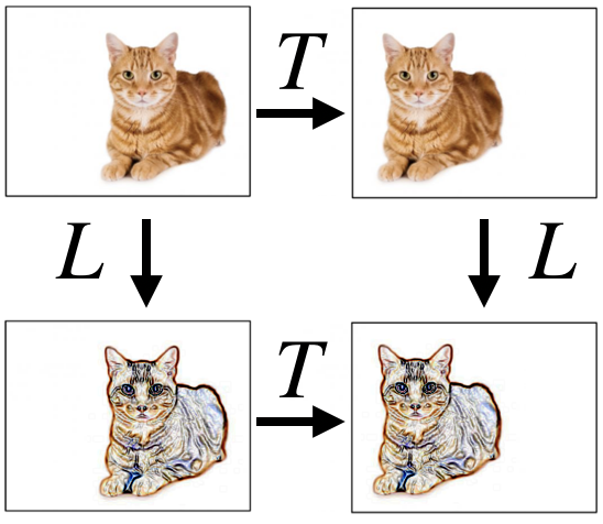
A much more useful idea is to think about equivariant linear operators, namely linear operators that commute with the translations (see image on the left), mathematically satisfying $L (T \cdot x)= T\cdot L(x)$ for all $x,T$. This condition implies that $A$ is a convolution operator (in fact, equivariance is a defining property of convolutions) and $b$ is a constant vector.

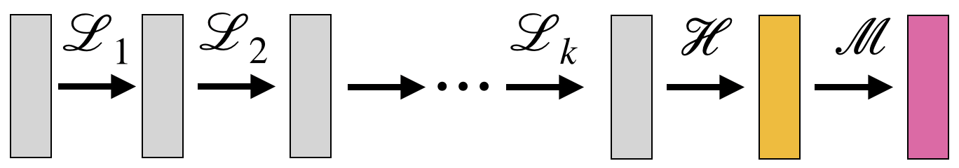
Now, a neural network defined by composing several equivariant layers $\mathcal{L}_i$, followed by a single invariant layer, $\mathcal{H}$, and an MLP, $\mathcal{M}$, namely $f(x)=\mathcal{M}\circ \mathcal{H}\circ \mathcal{L}_k\circ \cdots \circ \mathcal{L}_1(x)$ (see image), is by construction an invariant function and offers a much richer and expressive model that was used successfully to learn complicated image functions via Convolutional Neural Networks (CNNs) (Krizhevsky et al, 2012) that roughly follow this construction (the main difference is that CNNs usually use spatial pooling layers, that are not necessarily relevant for this note).

Representing graphs as tensors

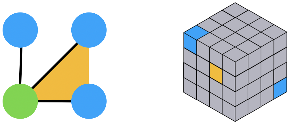
Instead of images, we would like to learn graphs, or more generally hypergraphs. Graphs and hypergraphs are mathematical objects that are widely used for representing structures ranging from social networks on the one hand, to molecules, on the other hand. A graph can be defined as a set of $n$ elements (nodes) for which we have some information $x_i$ attached to its i-th element, and some information attached to pairs of elements (edge), $x_{ij}$ will denote the information attached to the pair consisting of the i-th and j-th nodes. We will encode this data using a tensor $X\in\mathbb{R}^{n\times n}$, where the diagonal elements $X_{i,i} = x_i$ encode the node data and the off-diagonal elements, $X_{i,j} = x_{ij}$, $i\ne j$ , the edge data (for clarity, we discuss a single feature dimension).

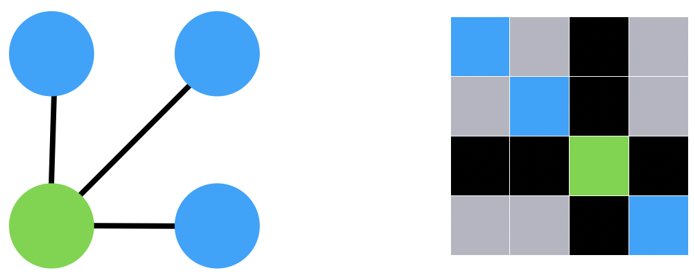
A natural generalization of a graph is a hypergraph where information is attached not only to single elements and pairs of elements but also 3-tuples, 4-tuples, or in general k-tuples. We represent such data using $X\in\mathbb{R}^{n^k}$, and each entry $X_{i_1,i_2,\ldots,i_k}$ represents the information of the corresponding k-tuple of elements. The figure above depicts a simple graph and its tensor representation (matrix). The figure below depicts a hypergraph of order 3 and its representing tensor.

Symmetries of graphs

Transformations that do “not change” the input data will be called symmetries. Translations are symmetries of images, but different kind of data, such as graphs may exhibit other symmetries. Note that in the representations of graphs introduced above, one can choose a different ordering of the set of nodes which affect the resulting tensor representation $X$.

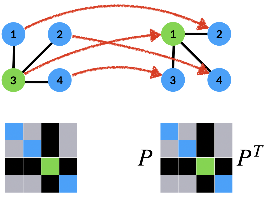
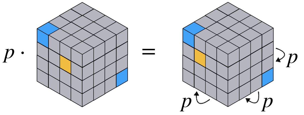
Two graphs $X,Y$ will be considered as the same (a.k.a. isomorphic) if there exists a permutation $p$ so that $Y=p\cdot X$, where $p\cdot X$ is a rearrangement of the rows and columns of $X$ according to $p$, that is, the $(i,j)$-th entry of $p \cdot X$ is $X_{p^{-1}(i),p^{-1}(j)}$. Using $p^{-1}$ and not $p$ in this definition is to make this action a left action, but is pretty arbitrary and does not really matter in our discussion. See the image above, where $P$ is the permutation matrix representing the permutation $p$. These symmetries generalize to hypergraphs where the permutation $p$ applied to all dimensions of $X\in\mathbb{R}^{n^k}$, namely the $(i_1,\ldots,i_k)$-th entry of $(p\cdot X)$ is $X_{p^{-1}(i_1),\ldots,p^{-1}(i_k)}$. This action is visualised for an example of a 3-order tensor in the figure below. Therefore, the symmetries of graph data are represented via the permutation group.

Invariant graph networks

We will use our understanding of the graph symmetries to come up with an effective inductive bias to learn graph data. That is, a way to restrict the linear transformations in the MLP so to achieve neural networks that are by construction invariant to the graph symmetries, without compromising the expressive power of the model. Similarly to the image case discussed above, trying to consider linear transformations of graph data $X\in\mathbb{R}^{n\times n}$ that are invariant, i.e., $L(p\cdot X) = L(X)$, leads to a poor space of operators: basically such $L$ are operators belong to a two-dimensional vector space containing summing the diagonal and summing the off diagonal of $X$. So for instance, networks using only such invariant layers could not distinguish two graphs if they have the same number of nodes and edges, which is of course not satisfying for learning interesting functions of graphs.
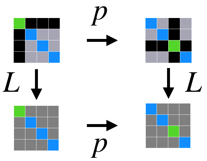
Exactly as in the image case, remedy comes from considering (the larger space of) equivariant operators, namely linear operators satisfying $L( p\cdot X) = p\cdot L(X)$ for all $p,X$. As for images, we will consider neural networks defined by composing several equivariant layers $\mathcal{L}_i$, followed by a single invariant layer, $\mathcal{H}$, and an MLP, $\mathcal{M}$, namely $f(X)=\mathcal{M}\circ \mathcal{H}\circ \mathcal{L}_k\circ \cdots \circ \mathcal{L}_1(X)$. $f$ is by construction an invariant function, namely satisfies $f(p\cdot X)=f(X)$. We call this network Invariant Graph Network (IGN) and discuss its properties next, but first we need to characterize the space of equivariant and invariant linear maps between tensors.

Note that in an IGN the hidden variables can be arbitrary tensors, $Y\in\mathbb{R}^{n^k}$ , even when the input tensors are of a lower order than $k$. Indeed, equivariant linear operators can map between different order tensors $\mathbb{R}^{n^k}\rightarrow \mathbb{R}^{n^l}$. For example, consider an IGN that receives an input graph tensor but learns information attached to triplets of nodes, then it would require a layer mapping order-2 tensor (i.e., matrix), $\mathbb{R}^{n^2}$, to order-3 tensor, $\mathbb{R}^{n^3}$. Another example is a network that takes in only set information (data only on nodes) in $\mathbb{R}^{n}$ and learns information on pairs of elements, $\mathbb{R}^{n^2}$. From now on, the term $k$-IGN will be used for describing an IGN with a maximal inner tensor degree of $k$.

Linear equivariant/invariant operators and the fixed point equations

We are looking to characterize affine transformations $\mathbb{R}^{n^k}\rightarrow \mathbb{R}^{n^l}$ equivariant ($l\geq 1$) or invariant ($l=0$) to the permutation action $X \mapsto p\cdot X$, as defined above. This is done in (Maron et al., 2019a) where the key idea is the following. Ignoring the constant part (i.e., bias) of $L$ (that can be treated in a similar way), a linear transformation $L:\mathbb{R}^{n^k} \rightarrow \mathbb{R}^{n^l}$ can be encoded as a tensor $L\in\mathbb{R}^{n^{k+l}}$. This is similar to a linear transformation $\mathbb{R}^k\rightarrow \mathbb{R}^l$ represented using a matrix in $\mathbb{R}^{k\times l}$. After applying some algebraic manipulations, the equations $L(p\cdot X) = p\cdot L(X)$ can be expressed compactly as $p\cdot L = L$; this includes both the case of linear equivariant operators ($ l\geq 1$), and linear invariant operators ($l=0$). We name these equations the fixed point equations as the space of equivariant/invariant operators $L:\mathbb{R}^{n^k} \rightarrow \mathbb{R}^{n^l}$ is characterized by all tensors $L\in\mathbb{R}^{n^{k+l}}$ that are fixed by the action of the permutation group .

How do we solve the fixed point equations? Any solution $L$ should be constant along orbits of the permutation group. For example, let us consider $k=l=2$, which corresponds to equivariant operators $\mathbb{R}^{n\times n}\rightarrow \mathbb{R}^{n\times n}$. If we consider $p=(12)$, that is, the permutation that interchanges 1 and 2 and keeps all other values in at place. Then, $L_{1,1,1,1}=p\cdot L_{1,1,1,1} = L_{p^{-1}(1),p^{-1}(1),p^{-1}(1),p^{-1}(1)}=L_{2,2,2,2}$. Similarly, considering $p=(23)$ we get $L_{2,2,2,2}=L_{3,3,3,3}$. Continuing in this manner we get that the diagonal $L_{i,i,i,i}$ is constant. Using a similar argument, one can see that $L_{1,1,2,3}$, for example, would equal all entries of the form $L_{i,i,j,s}$, where $i,j,s$ are all different. In general $L$ will be constant along indices $i,j,s,t$ that have the same equality pattern, that is, indices that preserve the equality and inequality relations between pairs. Therefore, the number of different orbits in this case will be the number of different equality patterns of four indices which equals the number of partitions of a set with four elements, also known as the Bell Number; in this case, $\mathrm{bell}(4)=15$. See image below.

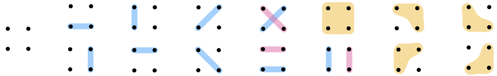
An orthogonal basis to the equivariant operators can, in turn, be constructed by considering an equality pattern ,$\alpha$, and the indicator tensor $B^\alpha_{i,j,s,t} = 1$ if and only if $(i,j,s,t)\in \alpha$ and $0$ otherwise. As shown in (Maron et al., 2019a) applying the equivariant operators can be done efficiently in $O(n^2)$ operations. As a result, a linear equivariant operator has the form $L = \sum_\alpha w_\alpha B^\alpha$, where $w_\alpha$ are the learnable parameters of the model. The figure illustrates the 15 different basis elements for $n=5, k=l=2$. Here, each square represents a matrix operating on the column stack of an $n\times n$ input tensor. Black pixels represent zero values, while white pixels represent the value 1.

In the general case, solving the fixed point equations for $l,k\in\mathbb{N}$ reduces to a fixed point equation for $L\in\mathbb{R}^{n^{k+l}}$. This equation can be solved by using the method above. In this case, we will have $\mathrm{bell}(k+l)$ basis elements (the number of equality patterns on $k+l$ indices) and the basis is given by the indicator tensors $B^\alpha$ of these equality patterns.

Remarks. (Maron et al., 2019a) can be seen as a generalization of Deep Sets (Zaheer et al., 2017, Qi et al,. 2017) that dealt with the case of node features and (Hartford et al., 2018) that studied equivariant layers for interaction between multiple sets. (Kondor et al., 2018) also identified several linear and quadratic equivariant operators and showed that the resulting network can achieve excellent results on popular graph learning benchmarks.

Bibliography

(Cybenko, 1989) Cybenko, G. (1989). Approximation by superpositions of a sigmoidal function. Mathematics of control, signals and systems, 2(4):303–314.

(Hartford et al., 2018) Hartford, J. S., Graham, D. R., Leyton-Brown, K., and Ravanbakhsh, S. (2018). Deep models of interactions across sets. In ICML.

(Hornik, 1991) Hornik, K. (1991). Approximation capabilities of multilayer feedforward networks. Neural networks, 4(2):251–257.

(Kondor et al., 2018) Kondor, R., Son, H. T., Pan, H., Anderson, B., and Trivedi, S. (2018). Covariant compositional networks for learning graphs. arXiv preprint arXiv:1801.02144.

(Krizhevsky et al., 2012) Krizhevsky, A., Sutskever, I., and Hinton, G. E. (2012). Imagenet classification with deep convolutional neural networks. In Advances in neural information processing systems, pages 1097–1105.

(Maron et al., 2019a) Maron, H., Ben-Hamu, H., Shamir, N., and Lipman, Y. (2019a). Invariant and equivariant graph networks. In International Conference on Learning Representations.

(Maron et al., 2019b) Maron, H., Fetaya, E., Segol, N., and Lipman, Y. (2019b). On the universality of invariant networks. In International conference on machine learning.

(Maron et al., 2019c) Maron, H., Ben-Hamu, H., Serviansky, H., and Lipman, Y. (2019c). Provably powerful graph networks. Advances in Neural Information Processing Systems.

(Qi et al., 2017) Qi, C. R., Su, H., Mo, K., and Guibas, L. J. (2017). PointNet: Deep learning on point sets for 3D classification and segmentation. In Proceedings - 30th IEEE Conference on Computer Vision and Pattern Recognition, CVPR 2017.

(Zaheer et al., 2017) Zaheer, M., Kottur, S., Ravanbakhsh, S., Poczos, B., Salakhutdinov, R. R., and Smola, A. J. (2017). Deep sets. In Advances in Neural Information Processing Systems, pages 3391–3401